Generating Synthetic Time Series with Diffusion Models

Cardiotocography (CTG) is a common way to monitor a baby during pregnancy and labor. Getting good CTG data for research is hard. It is sensitive, and the interesting cases are rare. Within the SECURED project, I built CTGen, an open-source framework that generates synthetic CTG with diffusion models. It was designed for CTG, but it works for any time series.

What is CTG?

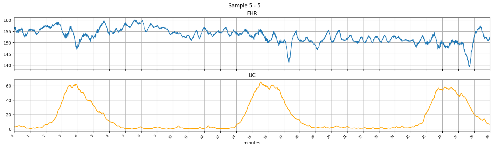
A CTG records two time series at the same time:

Fetal heart rate (FHR): the heart rate of the baby over time.
Uterine contractions (UC): the timing and intensity of the contractions.

A CTG recording

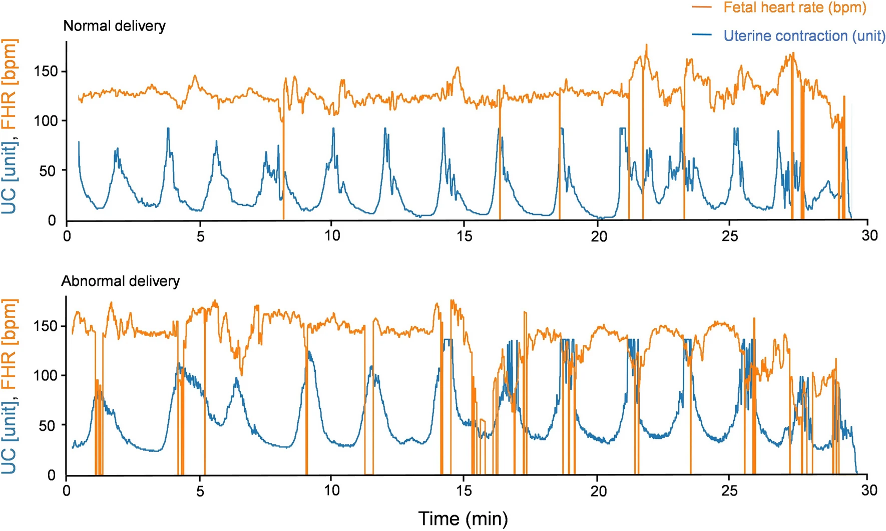
Doctors look at how the heart rate reacts to contractions. Certain patterns are signs of fetal distress, such as a lack of oxygen. Based on this, they decide whether to intervene, for example by inducing labor or performing a cesarean section.

Why generate synthetic CTG?

There are three potential use cases.

Data augmentation. Abnormal CTGs are much rarer than normal ones. Synthetic samples could balance a dataset and help train better classifiers.

Training human experts. Gynecologists and other professionals could learn from realistic examples that do not belong to any real patient.

Privacy. CTG alone may look harmless, but it can be combined with other data, such as hospital admission logs, timestamps or demographics. Then it can re-identify the mother or the baby. It can also reveal sensitive things: maternal conditions like diabetes or preeclampsia, the sex of the baby, or smoking and substance use inferred from heart rate variability. This puts CTG under regulations like GDPR, HIPAA and the EU AI Act. The concern is also not only about the mother and child, since such data can hint at genetic predispositions and family health information.

How diffusion models work here

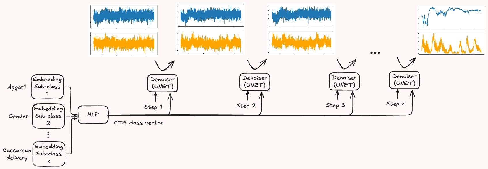
A diffusion model turns pure Gaussian noise into a realistic sample. It uses a denoiser, typically a U-Net, that predicts the noise in its input and removes it.

Training is simple. We add noise to a real CTG and give the noisy version to the U-Net. The clean CTG is the target. Removing all the noise in one step would be very hard, so the process is split into many small steps. One denoiser handles all steps, and the step number is an extra input.

CTG fits this setup well. The two signals (FHR and UC) become two input channels of the same length, like the RGB channels of an image. Just as neighboring pixels in an image are strongly correlated, neighboring time points in a CTG are too. This is why the convolutional U-Net works here with one small change. Images are 2D grids, so image U-Nets use 2D convolutions. A CTG channel is a 1D sequence over time, so we use 1D convolutions that slide along the time axis. The rest of the architecture stays largely the same.

Diffusion on CTG

Conditional generation

You often want a CTG with specific properties. The framework supports this with classifier-free guidance. Each sample can have several labels, such as delivery type, Apgar scores, the mother's age and the baby's sex. Unlike text prompts in image generation, these labels are discretized into categories, so each one is just an integer index. Each label gets its own embedding, the embeddings are combined into one vector, and this vector is an input of the U-Net. If you provide no labels, generation is unconditional.

Five ways to generate

A CTG recording is long, and generating long sequences directly is expensive. So the framework offers several strategies with different trade-offs. Every method is built from three configurable parts:

Compression (first_stage_model): how the time series is encoded into a latent space.
Denoising diffusion (ldm): the generative model that works in the output space of the compression.
Super-resolution (sr_model): an optional refinement step with its own compression model.

Mixing these gives the following methods.

1. Diffusion in the time domain

No compression. This is standard denoising diffusion: the model works directly on the raw data. This is simple and effective for shorter series or lower sampling frequencies. It becomes less scalable for long or high-resolution sequences.

2. Diffusion in the undersampled time domain

Keep only every $n$ -th sample (for example every 8th), run diffusion on this shorter signal, and scale the result back with linear interpolation. This is the fastest and simplest way to scale up. It needs no first-stage training. It works if the signal is redundant, so that downsampling loses little.

3. Learned compression

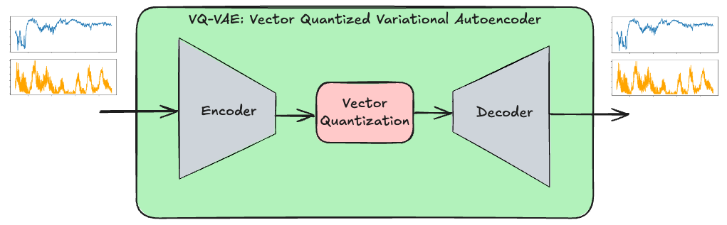
CTG is highly compressible because of its local correlation. A VAE, VQ-VAE or VQ-GAN can learn a compact latent space. Compared with naive downsampling, this gives higher compression, more accurate reconstruction, and features that can be useful for other tasks. Typical settings are small latent dimensions (2 to 4) and few layers (2 to 3) with many convolutional filters, to keep the local variations. The encoder is similar to the encoder half of the U-Net, and the decoder is its inverse.

Reconstruction uses an adjusted focal frequency loss, normalized separately for each channel because the channels have different scales and meaning. Unlike standard $L_{p}$ losses, it helps to preserve high-frequency components.

VQ-VAE

4. Latent diffusion

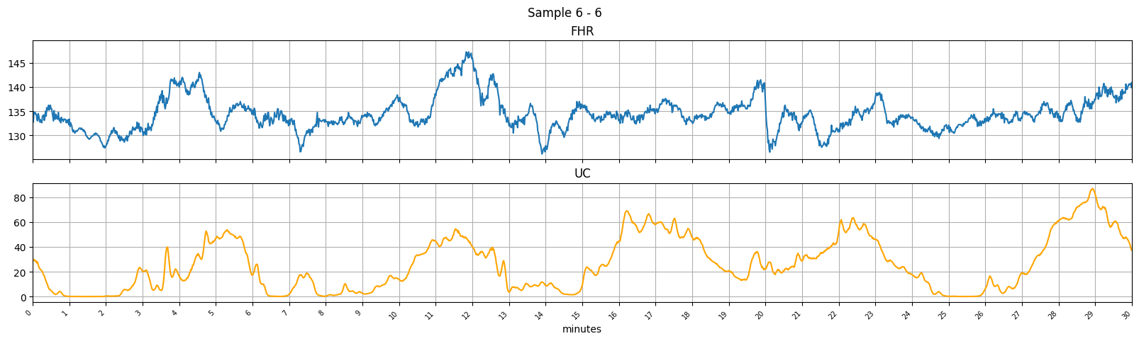
This is the same idea as Stable Diffusion. Train the first-stage model, then train the diffusion model on its latent space. To generate, sample a latent representation and decode it back to the time domain. The latent is much smaller than the signal, so this is significantly faster than generating in the time domain.

Sample generated with latent diffusion

5. Low-resolution diffusion plus latent super-resolution

This is a two-stage pipeline.

Stage one: a standard diffusion model generates an undersampled version of the CTG in the time domain. It captures the global trends and structure and ignores the fine, noisy details.

Stage two: a latent diffusion model upsamples the result. It is inspired by VQ-VAE-2 and the latent super-resolution of Stable Diffusion. The low-resolution signal is interpolated and encoded into a latent code $z_{l r}$ . A diffusion model then samples the high-resolution latent $z_{h r}$ . Its input is the concatenation of $z_{l r}$ and Gaussian noise along the channel dimension, so the fine details stay consistent with the coarse structure. Finally, a VQ-VAE decoder turns $z_{h r}$ into the full-resolution signal.

The idea is to generate the coarse structure first and add the detail afterwards. It costs two diffusion runs, but both work on small representations. Super-resolution can also be done in the time domain (identity first stage), but this is much slower for high-resolution series.

Sample generated with super-resolution

Features

General-purpose: it works with any multi-channel time series, not only CTG.
Modular: compression, diffusion and super-resolution are separate parts you combine in a YAML config.
Multiple compression options: identity, simple undersampling, VAE, VQ-VAE and VQ-GAN.
Conditional and unconditional generation: labels can come from a CSV file with the number of samples per label, or be sampled randomly from the training distribution.
Many samplers: DDPM, DDIM, PLMS, DPM-Solver and several samplers from k-diffusion.
Linear or cosine noise schedules.
Built-in evaluation: FID and Inception Score, plus classifier accuracy.

Data preparation

Each patient's CTG is a separate CSV file. The recording is cut into segments wherever the FHR stays at zero for longer than a set time, since this usually means the signal was lost. Training samples come from a sliding window over the segments. The data is scaled to $[- 1, 1]$ with min-max scaling and stored in PyTables together with the patient IDs, so labels can be linked to samples on the fly. I used the public Czech CTU-CHB dataset for the experiments, in this processed form.

Evaluation

FID and Inception Score need a classifier to extract features, and there is no standard one for CTG. The framework trains a fully convolutional network (FCN) for this. A separate classifier is trained for each label type, and the reported FID, IS and test accuracy are averages over them.

Privacy: synthetic does not mean safe

Synthetic data is often described as privacy-preserving. That is not automatically true. A generative model can memorize and leak information about its training data.

The standard way to test this is a membership inference attack (MIA). The attacker tries to decide whether a given sample was in the training set. We implemented LiRA (Likelihood Ratio Attack) against a model trained on the Czech dataset. It reached 70 to 80% accuracy, so the model does leak some information. I have not yet assessed a weaker black-box attacker who only sees the generated data.

Differentially private training (for example with Opacus) can reduce this risk, but it costs fidelity. Balancing the two is the interesting open question.

The code, configs and examples are on GitHub: github.com/gergelyacs/ctgen.

The code builds on several open-source projects, including lucidrains' denoising-diffusion-pytorch, PlantLDM, Stable Diffusion, k-diffusion, supervised-FCN-2, the focal frequency loss, and a processed CTU-CHB dataset. Full credits are in the README.